How to analyse excitons

In this tutorial you will learn (for a 2D-hBN) how to:

• analyze a BSE optical spectrum in terms of excitonic eigenvectors and eigenvalues
• look at the spatial distribution of the exciton

Prerequisites

Previous modules

• You must have completed the How to treat low dimensional systems tutorial

You will need:

• ypp executable
• xcrysden executable
• gnuplot or xmgrace executable

YAMBO calculations

If you have completed the tutorials of 2D hBN you should have all the databases required to do this tutorial in your SAVE and 2D directories

$ ls ./SAVE
ndb.gops ndb.kindx ns.db1  ns.kb_pp_pwscf_fragment_1 ....
$ ls ./2D
ndb.BS_Q1_CPU_0	ndb.cutoff	ndb.dip_iR_and_P_fragment_1	ndb.pp_fragment_1 ...

Sort the excitonic eigenvalues

$ ypp -e -s -J 2D 

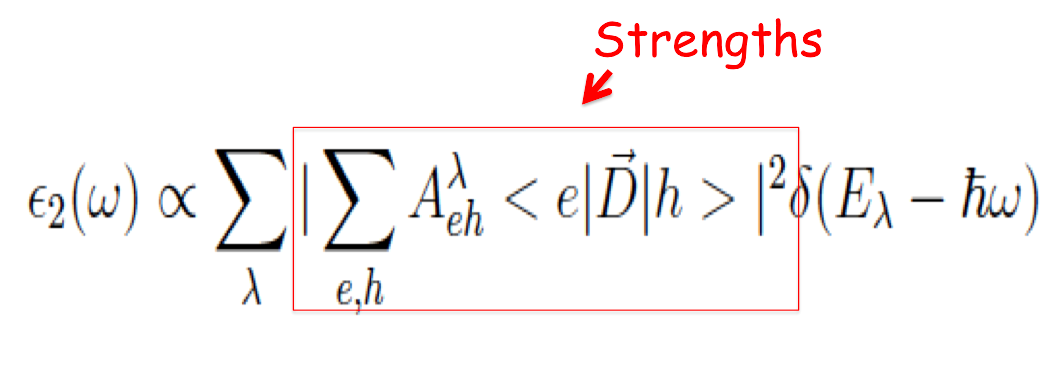
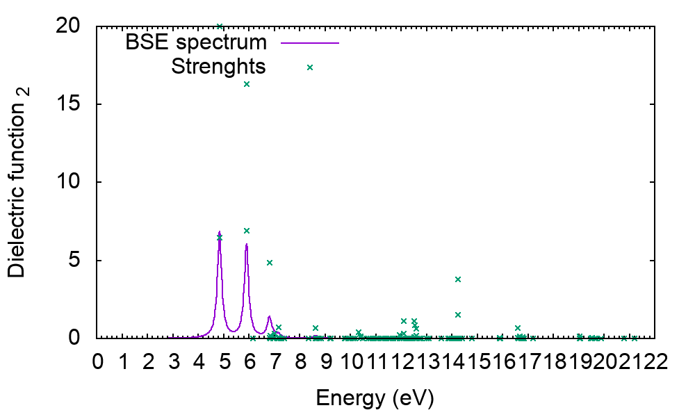
The new generated file o-2D.exc_I_sorted (o-2D.exc_E_sorted) reports the energies of the excitons and their Dipole Oscillator Strenghts sorted by energy (Index).

Open the first file and look inside. The first exciton is at 4.83 eV and the second one has the highest strenght (normalized to 1) Attention: clearly the convergence of these results has to be checked doing several BSE calculations with different k-grids!

Or you can make a plot

$ gnuplot
gnuplot> plot 'o-2D.eps_q1_diago_bse' w l title 'BSE2D' ,'o-2D.exc_E_sorted' u 1:($2*10) title 'Strenght2D'

Calculate the exciton oscillator strenght and amplitude

We can now analyze the excitons in terms of single-particle states, to do that create the appropriate input

$ ypp -e a -F ypp.AMPL.in -J 2D

Suppose you wish to analyze the first 5 excitons then change this line as:

States= "1 - 5"              # Index of the BS state(s)

Close the input and run ypp

$ ypp -J 2D -F ypp_AMPL.in

$ls ls o*exc*at*
o-2D.exc_amplitude_at_1 o-2D.exc_weights_at_1 ...

For an exciton [math]\displaystyle{ |\lambda\gt }[/math] , o-2D.exc_weights_at_* report the Weights

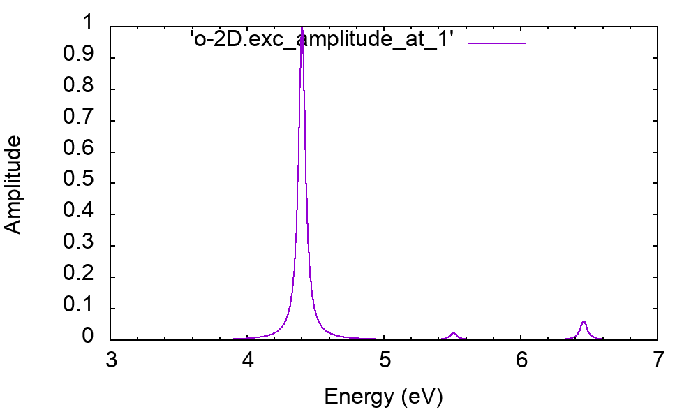
and o-2D.exc_amplitudes_at_* report the amplitudes

Open the file o-2D.exc_weights_at_1

#  Band_V     Band_C     K  ibz     Symm.      Weight     Energy
#
 4.000000   5.000000   7.000000   2.000000   0.922088   4.401093
 4.000000   5.000000   7.000000   1.000000    0.922081   4.401093

The first exciton is  essentially done of only single particle transitions from VBM to CBM at K (last k-point of the grid).

Plot the exciton spatial distribution

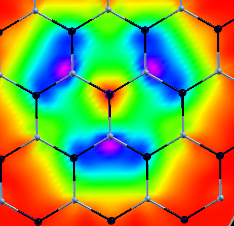
To see the spatial character of the exciton YPP fix the hole position and writes the electron spatical distribution probability. Different output formats can be selected and 1D,2D,3D plots done. Create the input and change the size of the cell where to see the exciton. Note that If the k-grid of the BSE simulation is a NxNx1 the exciton has an induced fictitious periodicity every Nx Nx1 Cell of the simulation. For hBN-2D this is not a problem because the exciton is strongly localized but in other systems with more delocalized excitons to look at the real exciton size it is necessary to use very large k-grids in the BSE

$ ypp -F ypp_WF.in -e w -J 2D 

excitons                     # [R] Excitons
wavefunction                 # [R] Wavefunction
Format= "x"                  # Output format [(c)ube/(g)nuplot/(x)crysden]
Direction= "12"               # [rlu] [1/2/3] for 1d or [12/13/23] for 2d [123] for 3D
FFTGvecs=  3951        RL    # [FFT] Plane-waves
States= "1 - 1"              # Index of the BS state(s)
Degen_Step=   0.0100   eV    # Maximum energy separation of two degenerate states
% Cells
 5 | 5 | 1 |                             # Number of cell repetitions in each direction (odd or 1)
%
% Hole
2.4     | 1.400     | 0.00     |        # [cc] Hole position in unit cell

Close the input and run ypp

$ ypp -F ypp_WF.in -J 2D

$ xcrysden --xsf o-2D.exc_2d_1.xsf